Jonathan Sedar
Personal website and new home of The Sampler blog
Bootstrapping Loss Ratios
Preamble
I currently work as a data scientist / statistician in commercial and specialty insurance. I’m not an actuary, just someone reasonably proficient with data analysis & modelling who saw (and continues to see) tremendous opportunities in the space.
I started to write a technical post about frequency-severity analysis of insurance claims using copulas to model the covariance: this yields a far better estimate of the expected loss cost and can thus guide pricing and portfolio performance measures.
Such analysis is really interesting and I feel doesn’t appear much in the literature, but assuming a mixed audience here of statisticians, actuaries and underwriters, I found that should first explain:
- loss ratios as point estimates and their general usage as the primary metric of underwriting performance
- why these point estimates are a poor qualifier of portfolio performance
- how we can make simple efforts to provide empirical probability distributions to qualify the point estimates
So let’s take a look at loss ratios and how to use bootstrapping (aka bootstrap resampling, sampling with replacement) to quickly and easily calculate empirical probability distributions to qualify these popular point-estimate portfolio performance metrics.
I’ve tried to make this post accessible to both underwriters and actuaries, so the math is light and I’ve omitted a lot of the code. Please stick with it and shout in the comments if you think this is wrong (!) or simply want a clearer explanation.
The briefest of primers on Loss Ratios
Insurance is an unusual good: the seller can never know the true cost of a policy before agreeing the contract.
Policy prices can be estimated using models based on historical outcomes of similar policies. The law of large numbers suggests that for a sufficiently decorrelated portfolio of policies, we ought to be able to offer similar premium prices for similar levels of policy coverage to similar insureds.
The loss ratio (LR) is simply the amount of claims (aka losses 1) paid out by the insurer divided by the premiums received from the insured: LR=Σ claimsΣ premiums
In the London market, insurance policies tend to run for one year of coverage, and syndicates will bundle them into a one-year portfolio or ‘binder’ according to their inception date. Broadly speaking, if a binder achieves a loss ratio LR≪100%, it means the insurer should be able to pay out all claims, collect a profit, and stay in business to provide the same service next year 2.
Premiums and claims amounts are conditional on time: the premium payments might be staggered over the policy term, and initial “incurred” claims amounts can grow over time as a claim event becomes more costly, or shrink as legal terms in a policy are arbitrated. Depending on the policy terms, valid liability claims might be reported during the in-force period of policy coverage “claims made”, or at some unknown point in future “occurence”.
These details & more mean that loss ratios are typically subtyped into a cornucopia of possibilities for “incurred but not (yet) reported”, “incurred but not enough reported”, “developed (forecasted) ultimate”, “true ultimate”, etc. All efforts so that (heavily regulated) insurance reserves can be closely monitored and managed. Final portfolio performance is typically presented only after some time: in the London Market the standard is to wait 3 years before accounting for a binder’s profit & loss.
Long after a claim is finally settled we might have a simple table of ultimate premiums and ultimate claims for each policy, and be able to calculate a very simple Ultimate Loss Ratio (ULR), for the portfolio.
e.g.
| policy_id | premium_amt | coverage | has_claim | claim_amt |
|---|---|---|---|---|
| p1 | $1000 | $100,000 | False | 0 |
| p2 | $1000 | $100,000 | True | $200 |
| p3 | $1200 | $150,000 | True | $600 |
Mean portfolio ULR=Σ((claim_amt))Σ(premium_amt)=$800$3200=25%
The performance of an insurance portfolio will typically be quoted as this single value point estimate ULR, very often without any attention to the distribution. It’s also common practice in commercial & specialty insurance to quote a premium price based on simple arithmetic - a rater - which is ‘targeted’ towards achieving such a point estimate, usually fitted to historical data or a synthetic portfolio.
Loss ratios have a great strength in that they’re very simple and intuitive: collect more money in reserves than you pay out, and you’ll probably turn a profit and stay in business
However, while these simple point-estimate sample mean loss ratios are not wrong per se, there are subtle issues with this naive approach:
- it’s not clear that the mean is a good summary statistic of the loss ratio distribution, which might easily be skewed (non-centred, asymmetrical)
- furthermore, in everyday life a mean value often implies a distribution that’s a sample from a random process with independent measurements i.e. a Gaussian, but there’s no reason to expect loss ratios to be Gaussian, so this is misleading
- relatedly, if an analyst does the unusual and provides a summary statistic of the spread of the distribution, it will likely be the variance or standard deviation, which also suggests a centered distribution with shallow tails, certainly not one with extreme kurtosis (fat tails)
- relatedly, the mean (and even variance if quoted) don’t say anything about the exceedance probability (EP) i.e. the probability that the loss ratio exceeds a certain value 3
- other issues include the glossing-over of sample sizes, statistical power, sample biases, latent probabilities, censoring, uncertainty propagation, prior assumptions, group effects and interactions, and any number of other fine details that would typically accompany a proper statistical explanation of claims phenomena.
It would be far more correct to undertake proper statistical modelling of portfolio & policy loss costs, broken down to claims frequency & severity, evidenced on observed & latent attributes of the insured risks and the loss-causing perils. I’ll write about that that soon.
Bootstrapping: Motivation and Concept
We have to accept that loss ratios are pervasive throughout the industry and serve reasonably well to let underwriters understand their book and set strategy for coverage terms, legal terms, pricing, risk selection, marketing and distribution. Without this, no business.
We also have no more data than the observed portfolio performance: there’s no meaningful counterfactuals, no randomised control trials to help determine causality, very little room for experimentation at all.
So perhaps we can at least work with the data we have, to quickly calculate the empirical distributions of the loss ratio from our sample, and use that to infer distribution in the universal population. Then we can better describe the portfolio performance in context.
Bootstrap resampling - “bootstrapping” - is based on the assumption that the observed data is an unbiased random sample from a wider ‘true’ population, and thus the variance within the observed data is representative of the variance within the wider population
The basic idea of bootstrapping is that inference about a population from sample data (sample → population) can be modelled by resampling the sample data and performing inference about a sample from resampled data (resampled → sample). As the population is unknown, the true error in a sample statistic against its population value is unknown. In bootstrap-resamples, the ‘population’ is in fact the sample, and this is known; hence the quality of inference of the ‘true’ sample from resampled data (resampled → sample) is measurable.
Worked example: Compare the means of two different arrays
Two equal-length arrays with the same mean but very different distributions
a = np.array([1, 1, 1, 1, 2, 2, 2, 2, 3, 3, 3, 3, 4, 4, 4, 4])
b = np.array([0, 0, 0, 0, 0, 0, 0, 0, 0, 0, 0, 8, 8, 8, 8, 8])
s = [(x.mean(), x.std()) for x in [a, b]]

print(f'a:  mean = {s[0][0]}, stdev = {s[0][1]:.2f}, unq = {np.unique(a)}')
print(f'b:  mean = {s[1][0]}, stdev = {s[1][1]:.2f}, unq = {np.unique(b)}')
a:  mean = 2.5, stdev = 1.12, unq = [1 2 3 4]
b:  mean = 2.5, stdev = 3.71, unq = [0 8]
Observe:
-
Both arrays have a mean (Expected value) of 2.5,
- For
a, the mean 2.5 is close to the observed values (the centre in fact) - But for
b, mean 2.5 is far from the observed values and is a poor predictor of values
- For
-
The standard deviations (s.d.) are very different: 1.12 and 3.71 respectively
- For
a, values within the span of 1 s.d. or 2 s.d. are actually seen in the data - But for
b, only one observed value (0) is within 1 s.d. of the mean, and the 1 s.d. width pushes negative forcing us to question whether negative values are even allowed in our data generating process
- For
We could represent the arrays using e.g. a histogram or kde, but that still doesn’t tell us about the variance in the true population, and the variance in any summary statistic.
…What we really want are distributions in the summary statistics
The bootstrapping process is really simple:
- For each array length
n, sample with replacement to create a new array lengthr. - Calculate and record the summary statistic of choice (here, the mean).
- Repeat this
n_bootstrapstimes to get a new array of resample means with lengthn_bootstraps - Evaluate the distribution of this new array
A really quick aside on r
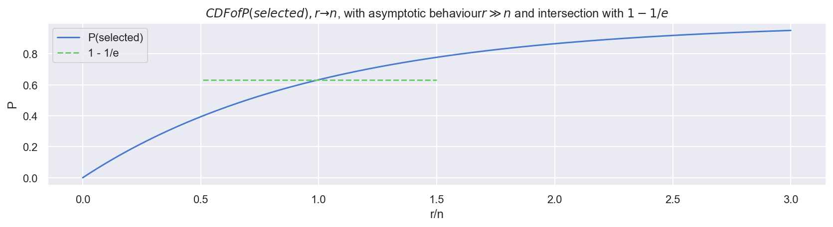
Convention is to set the number of resamples r the the same size as the original array: r∼n. This preserves the sample error in the resamples, and allows the resample to behave with the same variance as the sample.
Interestingly (inevitably), r→n has a direct relationship to stopping problems:
- Within a sample of size n, the probability of any one item being selected into resample (with replacement) r, is P(selected)=1−(1−1n)r
- As you can see in the following plot, in the limit limr→n,P(selected)→1−1e
- This equivalent to the probability of rejecting the best candidate in the secretary problem
Back to it: Bootstrap resample both arrays, and view the distribution of the mean
Use numpy broadcasting (vectorised, very quick) to create a 2D array of bootstraps * resamples
rng = np.random.default_rng(42)
n_bootstraps = 50
r = len(a)
boot_a = rng.choice(a, size=(n_bootstraps, r), replace=True)
boot_b = rng.choice(b, size=(n_bootstraps, r), replace=True)

dfbootmean = pd.DataFrame({'boot_a_mean': boot_a.mean(axis=1),
                           'boot_b_mean': boot_b.mean(axis=1)})
dfbootmean.mean()
boot_a_mean    2.52125
boot_b_mean    2.50000
dtype: float64
Observe:
- For each array, the mean of the bootstrap means is similar to the straight sample mean (2.5)
- But it isn’t identical, and
adiffers fromb - To understand this in more detail, plot the distributions of bootstrap means
Plot distributions of resample means
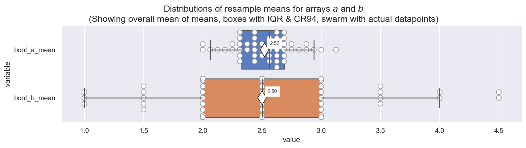
(If you’re not familiar with boxplots, note the 50% Credible Region (CR50 aka Interquartile Range aka IQR) at the (25,75) percentiles, and the 94% Credible Region (CR94) at the (3, 97) percentiles. The CR50 contains 50% of the distribution, and the CR94 contains 94%)
Observe:
- These distributions of resample (bootstrap) means put the sample means into context
- We easily see that
boot_a_meanhas a narrower, more centered distribution with a similar mean and median, and a smoother distribution of values - Conversely,
boot_b_meanhas a wider, skewed distribution with kurtosis and strong quantisation of values implying relative instability of the mean estimate - Now we can state expected values with qualification:
ahas population mean 2.52 with CR94 (2.1, 2.9)bhas population mean 2.50 with CR94 (1.0, 4.5)- in fact the CR94 for
afits completely within the CR50 ofb!
- We should put much less credibility on the population mean for
b - If we have to predict the next value in each array, we will have far more
credibility in our predictions for
a, than forb
Create a Synthetic Portfolio
Now let’s make this relevant to the task at hand: estimating variance in portfolio loss ratios.
Imagine we’re an MGA underwriting policies on behalf of a regulated insurer for a fairly simple commercial & specialty product: Professional Indemnity (PI) for Small-Medium Enterprises (SMEs). This might cover IT contractors, accountants, engineers, solicitors etc. for their client’s damages stemming from poor advice and/or deliverables, with a typical exposure limit around $5M.
We’ll create a broadly realistic dataset of exposure, premiums and claims:
- The exposure is a biased sample of limits between $1M and $5M
- The premium is a simple, static “rate-on-line” of 0.1% of exposure, with some added noise to simulate a price created via a marginalized risk tuning (rater)
- We assume a maximum of one claim per policy
- The claims generating process is modelled as:
- a latent probability of making a claim
- a conditional latent probability of the claim severity (measured as losses per unit exposure)
rng = np.random.default_rng(42)
n_policies = 5000
rate_on_line = 5e-3

dfc = pd.DataFrame({'policy_id': [f'p{i}' for i in range(n_policies)],
                    'exposure_amt': rng.choice([1e6, 2e6, 3e6, 5e6],
                                               p=[0.1, 0.3, 0.2, 0.4], size=n_policies)})
dfc.set_index('policy_id', inplace=True)

dfc['premium_amt'] = (np.round(dfc['exposure_amt'] /
                      rng.normal(loc=1/rate_on_line, scale=25, size=n_policies), 2)

dfc['latent_p_claim'] = rng.beta(a=1, b=150, size=n_policies)
dfc['latent_p_sev'] = rng.gamma(shape=1.5, scale=0.25, size=n_policies)

dfc['has_claim'] = rng.binomial(n=1, p=dfc['latent_p_claim'])
dfc['claim_amt'] = dfc['has_claim'] * dfc['latent_p_sev'] * dfc['exposure_amt']

print(f'\n{n_policies} policies, ${dfc["exposure_amt"].sum()/1e9:.1f}B exposure, ' +
      f'${dfc["premium_amt"].sum()/1e6:.1f}M premium, with {dfc["has_claim"].sum():.0f} claims ' +
      f'totalling ${dfc["claim_amt"].sum()/1e6:.1f}M. ' +
      f'\n\n ---> yielding an observed portfolio LR = {dfc["claim_amt"].sum() / dfc["premium_amt"].sum():.1%}')
5000 policies, $16.4B exposure, $83.3M premium, with 38 claims totalling $44.5M.

 ---> yielding an observed portfolio LR = 53.3%
Observe:
- This dataset is randomly generated, but is a reasonably realistic 1-year portfolio for a small MGA
- With a Loss Ratio of 53%, the insurer can pay out all the claims and stay in business next year (again we ignore the Combined Ratio for this exercise)
Summarise claims activity
def summary_stats(s):
    return pd.Series({'count': len(s), 'sum': np.sum(s), 'mean': np.mean(s)})

dfc.groupby('has_claim').apply(lambda g: summary_stats(g['claim_amt']))
| count | sum | mean | |
|---|---|---|---|
| has_claim | |||
| 0 | 4962.0 | 0.000000e+00 | 0.000000e+00 |
| 1 | 38.0 | 4.445095e+07 | 1.169762e+06 |
Observe:
- This portfolio experienced 38 claims over the year, not unrealistic for PI coverage - which tends to have fewer, more severe claims
- The total claims is ~ $44M, with a mean claim payout ~ $1M
So, can we leave it there?
We seem to have underwritten a successful portfolio, can we grow the business and take on more risk next year? Perhaps we can also charge the insurer a higher underwriting fee?
Not so fast…
- What if we had written an ever-so slightly different portfolio - would it have arrived at a very different (mean) LR?
- In fact, is the mean LR overly influenced by a few outlier policies?
- What’s the uncertainty in our predictions for next year’s portfolio performance?
We can’t yet evaluate the mean in context of the wider population, so let’s bootstrap!
Bootstrapping to Evaluate Loss Ratios
Use the same bootstrap resampling concept as above, to sample-with-replacement many slightly different variations of our observed portfolio
Example 1: Simple Loss Ratio Variance over an entire Portfolio
def bootstrap_lr(df, nboot=1000):
    """
        Convenience fn: vectorised bootstrap for df
        uses numpy broadcasting to sample
    """
    rng = np.random.default_rng(42)

    sample_idx = rng.integers(0, len(df), size=(len(df), nboot))
    premium_amt_boot = df['premium_amt'].values[sample_idx]
    claim_amt_boot = df['claim_amt'].values[sample_idx]

    dfboot = pd.DataFrame({
                'premium_amt_total_pb': premium_amt_boot.sum(axis=0),
                'claim_amt_total_pb': claim_amt_boot.sum(axis=0)})

    dfboot['lr_pb'] = dfboot['claim_amt_total_pb'] / dfboot['premium_amt_total_pb']

    return dfboot
dfc_boot = bootstrap_lr(dfc)
dfc_boot.head(3)
| premium_amt_total_pb | claim_amt_total_pb | lr_pb | |
|---|---|---|---|
| 0 | 8.340700e+07 | 4.865762e+07 | 0.583376 |
| 1 | 8.425466e+07 | 2.959219e+07 | 0.351223 |
| 2 | 8.291968e+07 | 4.667287e+07 | 0.562868 |
Observe:
- This code creates 1000 bootstrap resamples, each a variant of our original portfolio
- (The first 3 rows of the resamples are shown above)
- We sum the premium and claims amounts for each portfolio and calculate a loss ratio
- Now we have 1000 slightly different realisations of the portfolio loss ratio
- The mean of these realisations will tend towards the sample mean, and the variance on the mean will reflect the variance in the wider ‘true’ population
View distribution of bootstrap-resampled loss ratio
Empirical PDF
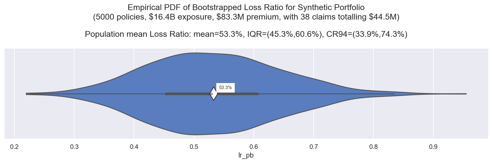
Observe:
- The mean of our bootstrap mean LR (approx the population mean) is 53.3%, the same as the sample mean LR
- Now variance in the bootstrap means shows us the variance in that sample mean: ranging IQR=(45%, 61%) and CR94=(34%, 74%)
- This is quite a wide range, indicating low stability in the portfolio performance,
Now we can state our portfolio LR within a range of credibility:
- The experienced, observed portfolio LR is 53%
- If this portfolio is representative of the portfolio we plan to write next year
and we believe it to perform in a similar way, then the inherent variance tells
us that next year’s portfolio LR will land:
- between (45%, 61%) with 50% confidence
- between (34%, 74%) with 94% confidence
To continue this train of thought, it is very important for business planning to estimate the probability of exceeding a certain LR, so we can easily turn this into an “exceedance curve”.
Empirical Survival Curve (1 - CDF) aka Exceedance Curve
We can read this curve vertically to determine the empirical probability of achieving a particular LR, or horizontally to see the LR at a 1-in-X years frequency
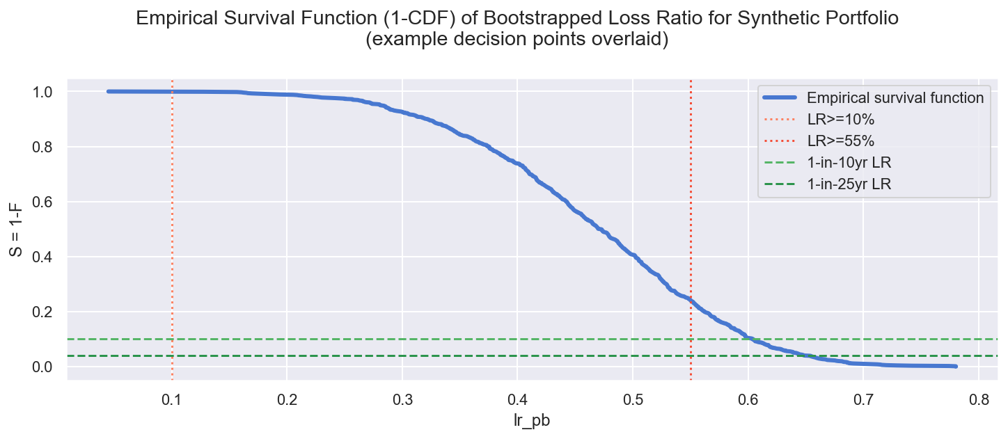
LR>10% = 99.9%
LR>55% = 24.1%
1-in-10yr LR = 60.4%
1-in-25yr LR = 64.9%
Observe:
Reading vertically we can address e.g.:
-
The regulator requires a 10% minimum loss ratio to assure our product is not overpriced:
- Question: What’s the probability of our portfolio yielding an LR>10%?
- Answer:
(lr_pb = 0.1: P ~ 0.999): close to 100%, almost certain
-
Our total cost of business adds 40pts to the Combined Ratio, our reinsurance treaty kicks in above 95%:
- Question: What’s the probability the LR exceeds 55%?
- Answer:
(lr_pb = 0.55: P ~ 0.24): at 24% it appears unlikely that the reinsurance treaty will be triggered, but this might encourage us to reduce the cost of business and/or renegotiate the reinsurance deal
Reading horizontally we can address e.g.:
-
We require our capital reserves to easily withstand a 1-in-10 year loss:
- Question: What’s our expected 1-in-10 year worst Loss Ratio?
- Answer:
(P = 0.1: lr_pb = 0.604): we expect the worst 1-in-10 year LR∼61%
-
We also require our capital reserves to withstand a 1-in-25 year shock result:
- Question: What’s our expected 1-in-25 year worst Loss Ratio?
- Answer:
(P = 0.04: lr_pb = 0.649): we expect the worst 1-in-25 year LR∼65%
Example 2: Comparison between sub-groups within a Portfolio
Now let’s compare the performance of different parts of the portfolio - perhaps to influence risk selection, or justify a longer project plan to adjust the pricing model. Of course, the same principle applies to comparing portfolios.
For convenience here I’ll split by exposure band, but note this is not strictly an inherent property of the insured (although no doubt correlated) so in practice this would be a less useful split than e.g. insured business size or location
dfcg_boot = dfc.groupby('exposure_amt').apply(bootstrap_lr)
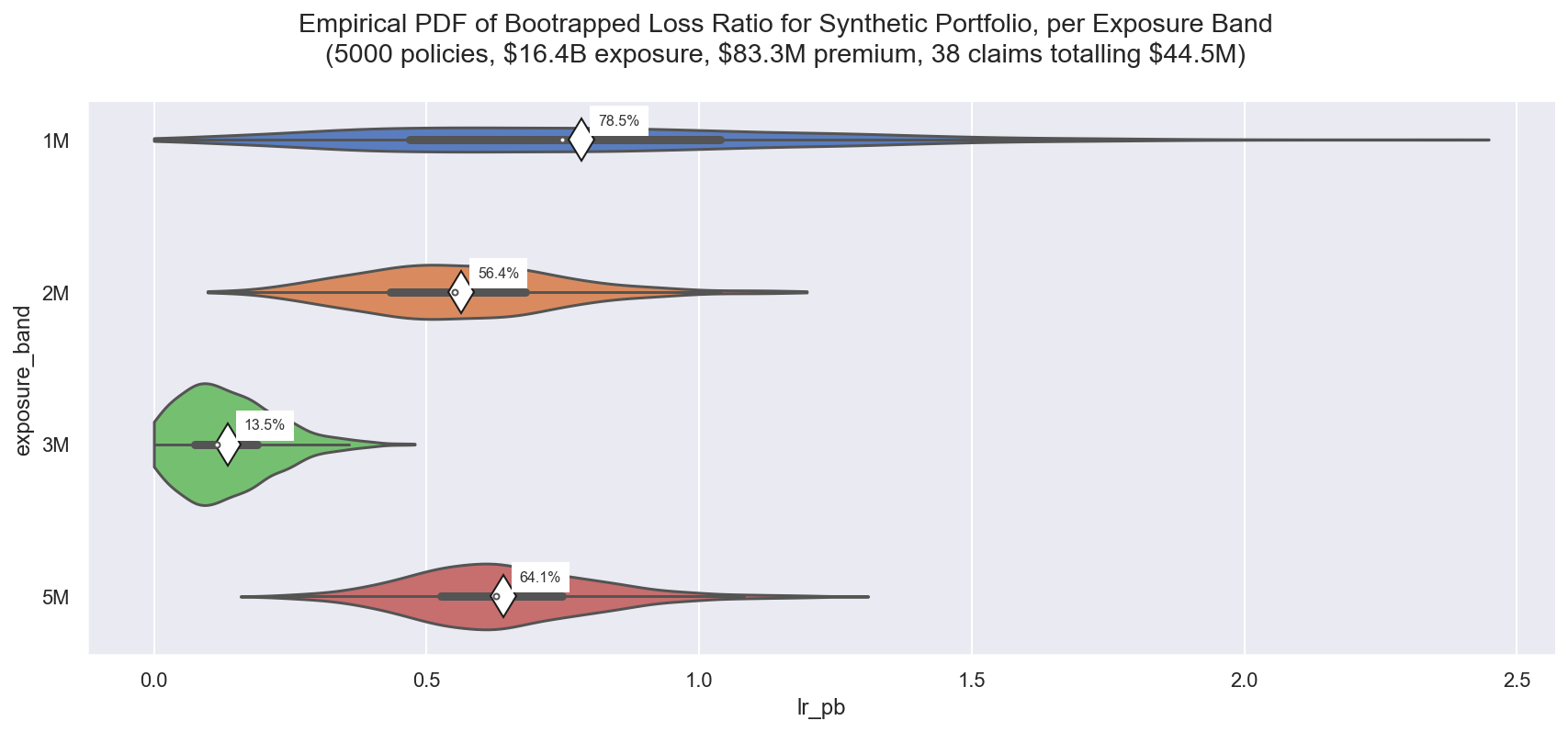
Observe:
- Here we see some very large differences in the empirical PDFs of LR between the exposure bands
- Band $1M has far greater variance than the rest, in the real world this would be a clear alert to investigate and try to reduce the volatilty, perhaps through better risk selection or finer-tuned pricing
- Band $3M has a smaller variance and lower LR than the rest - in the real world this also would be a clear alert to investigate further, try to understand why the performance is so good, and perhaps adjust underwriting accordingly to attract more of this type of insured
3.2.1 Compare difference between the distributions (BEST)
In the above plot, exposure band $5M appears to perform worse (have a higher LR) than exposure band $2M.
Because we have the full bootstrap resample distributions available, we can approximate a probabilistic comparison to ask “does exposure band $5M perform credibly worse than band $2M?"
This is loosely equivalent to
John Krushke’s BEST model
(Bayesian Estimation Supersedes the T-Test)
(find an implementation in the pymc3 docs).
BEST is similar in spirit (though different in practice), to the concept of
frequentist null hypothesis testing, wherein strong assumptions of distributional
form and asymptotics are used to state the ‘statistical’ difference between
distributions, often quoted as a p-value. This BEST method dispenses with the
asymptiotic assumptions and idealised scenarios to consider only the empirical
observations at hand.
What we’re looking for is the distribution of the simple elementwise difference between the distributions. We can state the credibility of the difference w.r.t a reference value of zero: if the distribution of differences lies far from zero, then there is a credible difference between the portfolios.
idx2 = dfcg_boot['exposure_band']=='2M'
idx5 = dfcg_boot['exposure_band']=='5M'
delta_5m2 = dfcg_boot.loc[idx5, 'lr_pb'].values - dfcg_boot.loc[idx2, 'lr_pb'].values
prop_lt0 = sum(delta_5m2 < 0) / len(delta_5m2)
txtcred = 'not ' if 1 - np.abs(prop_lt0) > 0.05 else ''
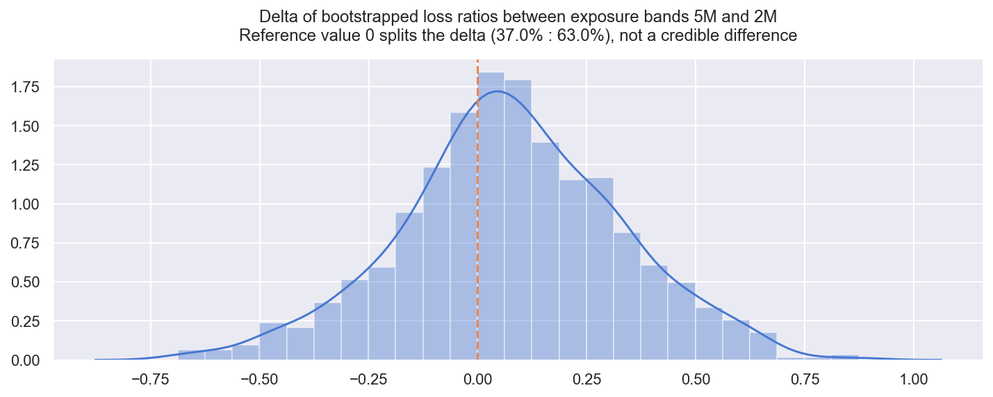
Observe:
- Despite the mean LRs looking quite different ($5M has 64.1% LR, and $2M has 56.4%LR) the difference between the bootstrapped distributions of the mean is split 37:63
- This means that the $5M exposure band has a higher LR (performs worse) in only 63% of the bootstrap resamples
- We might choose to set a level of credibility at 95% (comparable to the completely arbitrary p=0.05 in a t-test), in which case our observed difference of 63%, is not credible, and in the real world we could not support decisions to treat these bands differently
Quick Recap
We covered:
- The core concept of a loss ratio and why they are pervasive throughout insurance
- Why this summary statistic is a poor estimate of the variance in a portfolio and a poor predictor for the loss ratio of future portfolios
- How we can (and should) make use of bootstrap resampling to very quickly & easily estimate the loss ratio variance in a portfolio and put our sample mean into context of the population mean
- How we can use these bootstrap resamples to report various probabilistic statements e.g.: a. the probability of the loss ratio exceeding a desired value b. the probable loss ratio at a desired reoccurence rate c. the probabilistic difference between two portfolios (or sub-portfolios)
Most important to remember is that bootstrapping is simple and powerful. It has a part to play in all exploratory data analysis.
-
Yes… I know. ↩︎
-
Here I ignore broker fees, claims arbitration, reinsurance, costs of business and investment returns. That grand total is the Combined Ratio which in practice, can often run close to or over 100% ↩︎
-
Interestingly, due to the extreme skew and kurtosis in natural catastrophe events, it’s common to report cat modelling results as EP curves. ↩︎