Jonathan Sedar
Personal website and new home of The Sampler blog
PyMC3 Examples: GLM with Custom Likelihood for Outlier Classification
Preamble
I first created this content at the end of 2015 and submitted to the examples documentation for the PyMC3 project and presented a version at our inaugural Bayesian Mixer London meetup. The presentation wasn’t much more than an attempt to get the ball rolling, but it must have done something right since the meetup is still going strong. A record of the evening appears to survive on Markus Gessman’s blog.
The Notebook received an update in 2018 from
Thomas Wiecki -
reworking the specification for the Hogg model ‘Signal vs Noise’ to use a
pm.Potential instead of the rather verbose custom likelihood written in
theano. That v2.0 of the Notebook is
available in the project examples documentation.
I recently revisited this code and realised a lot has changed since 2015, so
I’ve given it a thorough spring clean and pushed a
v2.1 of the Notebook up on Github.
This version is developed against python3.6 and pymc3.7, contains a more
efficient StudentT model, uses the pm.Data object, and contains plate
notation, updated arviz plots and explanations throughout.
It’s hard to find time for the study required to make fundamental contributions
to the PyMC3 (and now PyMC4) projects, but if I can submit examples for how to
use the library, then all the better. So this Notebook is re-hosted in a new
personal repo I’ve created specifically for my
pymc3_examples.
It’s simple to reproduce the self-contained project setup using the README,
and the conda env and pip instructions and the README, and the license
is MIT. This new submission is currently pending a PR, and I’ll note here
if/when it’s accepted.
GLM with Custom Likelihood for Outlier Classification (Abridged)
This content is condensed from a far more detailed Notebook up on Github which is designed to be fully reproducible in an MVP environment or standalone. The following content has been heavily abridged so we can get to the models, if something doesn’t make sense then please see the full Notebook.
The general concept is to filter out noisy / erroneous datapoints in a set of observations. We propose that a main set of ‘inliers’ are created by a particular model that we specify and a set of ‘outliers’ that fit better to some alternative model.
This implementation is a copy of eqn 17 in Hogg et al. (2010) Data analysis recipes: Fitting a model to data, and is adapted specifically from Jake Vanderplas' implementation for the AstroML book:
- it was created to separate signal vs noise in a set of astronomical observations
- it relies on a Bernoulli assignment of each datapoint to switch between an inliers ‘signal’ model (based on a theoretical set of relationships), or an outliers ‘noise’ model (based on unknown variance)
- it marginalizes over the probability that a datapoint is an outlier, converging to a posterior joint distribution where inliers and outliers are fitted best.
It’s interesting to note the domain specificity and weaknesses of this implementation:
- the hard-scientific domain leads us to test the validity of a well-posed theoretical model and have no room for subjectivity: so an observation either fits the theory or must be due to measurement error
- this is a very strong statement for wider application in use in softer sciences and humanities domains
- the model can easily suffer from instabilities when sampling, and we’ll see in a future notebook how to alternatively treat this as a soft mixture model.
Contents
- 1. Basic EDA
- 2. Basic Feature Engineering
- 3. Simple Linear Model with no Outlier Correction
- 4. Simple Linear Model with Robust Student-T Likelihood
- 5. Linear Model with Custom Likelihood to Distinguish Outliers: Hogg Method
1. Basic EDA
1.1 Load Data
The dataset is available within AstroML and since it’s a very small dataset, is hardcoded below
# cut & pasted directly from the fetch_hogg2010test() function
# identical to the original dataset as hardcoded in the Hogg 2010 paper

dfhogg = pd.DataFrame(
                np.array([[1, 201, 592, 61, 9, -0.84],
                          [2, 244, 401, 25, 4, 0.31],
                          [3, 47, 583, 38, 11, 0.64],
                          [4, 287, 402, 15, 7, -0.27],
                          [5, 203, 495, 21, 5, -0.33],
                          [6, 58, 173, 15, 9, 0.67],
                          [7, 210, 479, 27, 4, -0.02],
                          [8, 202, 504, 14, 4, -0.05],
                          [9, 198, 510, 30, 11, -0.84],
                          [10, 158, 416, 16, 7, -0.69],
                          [11, 165, 393, 14, 5, 0.30],
                          [12, 201, 442, 25, 5, -0.46],
                          [13, 157, 317, 52, 5, -0.03],
                          [14, 131, 311, 16, 6, 0.50],
                          [15, 166, 400, 34, 6, 0.73],
                          [16, 160, 337, 31, 5, -0.52],
                          [17, 186, 423, 42, 9, 0.90],
                          [18, 125, 334, 26, 8, 0.40],
                          [19, 218, 533, 16, 6, -0.78],
                          [20, 146, 344, 22, 5, -0.56]]),
                columns=['id','x','y','sigma_y','sigma_x','rho_xy'])

dfhogg['id'] = dfhogg['id'].apply(lambda x: 'p{}'.format(int(x)))
dfhogg.set_index('id', inplace=True)
dfhogg.head()
| x | y | sigma_y | sigma_x | rho_xy | |
|---|---|---|---|---|---|
| id | |||||
| p1 | 201.0 | 592.0 | 61.0 | 9.0 | -0.84 |
| p2 | 244.0 | 401.0 | 25.0 | 4.0 | 0.31 |
| p3 | 47.0 | 583.0 | 38.0 | 11.0 | 0.64 |
| p4 | 287.0 | 402.0 | 15.0 | 7.0 | -0.27 |
| p5 | 203.0 | 495.0 | 21.0 | 5.0 | -0.33 |
1.2 Exploratory Data Analysis (Trivial)
Just a quick plot to aid understanding
- the dataset contains errors in both the x and y, but we will deal here with only errors in y.
- see the Hogg 2010 paper for detail
gd = sns.jointplot(x='x', y='y', data=dfhogg, kind='scatter', height=8,
        marginal_kws={'bins':12, 'kde':True, 'kde_kws':{'cut':1}},
        joint_kws={'edgecolor':'w', 'linewidth':1.2, 's':80})

_ = gd.ax_joint.errorbar('x', 'y', 'sigma_y', 'sigma_x', fmt='none',
                            ecolor='#4878d0', data=dfhogg, zorder=10)
for idx, r in dfhogg.iterrows():
    _ = gd.ax_joint.annotate(s=idx, xy=(r['x'], r['y']), xycoords='data',
                             xytext=(10, 10), textcoords='offset points',
                             color='#999999', zorder=1)

_ = gd.annotate(stats.pearsonr, loc="upper left", fontsize=12)
_ = gd.fig.suptitle(('Original datapoints in Hogg 2010 dataset\n' +
        'showing marginal distributions and errors sigma_x, sigma_y'), y=1.05)
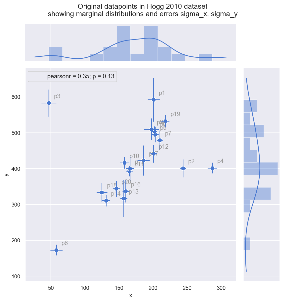
Observe:
- just by eye, you can see these observations mostly fall on or around a straight line with positive gradient
- it looks like a few of the datapoints (
p2,p3,p4, maybep1) may be outliers from such a line - measurement error (independently on x and y) varies across the observations
2. Basic Feature Engineering
Ordinarily we would run through more formalised steps to split into Train and Test sets (to later help evaluate model fit), but here I’ll just fit the model to the full dataset and stop at inference
2.1 Transform and standardize dataset
It’s common practice to standardize the input values to a linear model, because this leads to coefficients sitting in the same range and being more directly comparable. Gelman notes this in a 2007 paper.
So, following Gelman’s paper above, we’ll divide by 2 s.d. here:
- since this model is very simple, we just standardize directly, rather than
using e.g. a scikit-learn
FunctionTransformer - ignoring
rho_xyfor now
Additional note on scaling the output feature y and measurement error
sigma_y:
- This is unconventional - typically you wouldn’t scale an output feature
- However, in the Hogg model we fit a custom two-part likelihood function of
Normals which encourages a globally minimised log-loss by allowing outliers to
fit to their own Normal distribution. This outlier distribution is specified
using a stdev stated as an offset
sigma_y_outfromsigma_y - This offset value has the effect of requiring
sigma_yto be restated in the same scale as the stdev ofy
Standardize (mean center and divide by 2 sd)
dfhoggs = ((dfhogg[['x', 'y']] - dfhogg[['x', 'y']].mean(0)) /
           (2 * dfhogg[['x', 'y']].std(0)))
dfhoggs['sigma_x'] = dfhogg['sigma_x'] / ( 2 * dfhogg['x'].std())
dfhoggs['sigma_y'] = dfhogg['sigma_y'] / ( 2 * dfhogg['y'].std())
3. Simple Linear Model with no Outlier Correction
3.1 Specify Model
Before we get more advanced, I want to demo the fit of a simple linear model with Normal likelihood function. The priors are also Normally distributed, so this behaves like an OLS with Ridge Regression (L2 norm).
Note: the dataset also has sigma_x and rho_xy available, but for this exercise, I’ve chosen to only use sigma_y
ˆy∼N(βT→xi,σi)
where:
- β = {1,βj∈Xj} <— linear coefs in Xj, in this case
1 + x - σ = error term <— in this case we set this to an unpooled σi: the measured error
sigma_yfor each datapoint
with pm.Model() as mdl_ols:

    ## Define weakly informative Normal priors to give Ridge regression
    b0 = pm.Normal('b0_intercept', mu=0, sigma=10)
    b1 = pm.Normal('b1_slope', mu=0, sigma=10)

    ## Define linear model
    y_est = b0 + b1 * dfhoggs['x']

    ## Define Normal likelihood
    likelihood = pm.Normal('likelihood', mu=y_est, sigma=dfhoggs['sigma_y'],
                           observed=dfhoggs['y'])

pm.model_to_graphviz(mdl_ols)

3.2 Fit Model
3.2.1 Sample Posterior
with mdl_ols:
    trc_ols = pm.sample(tune=5000, draws=500, chains=3, cores=3,
                    init='advi+adapt_diag', n_init=50000, progressbar=True)
Auto-assigning NUTS sampler...
Initializing NUTS using advi+adapt_diag...
Average Loss = 150.96:  20%|█▉        | 9871/50000 [00:06<00:26, 1516.47it/s]
Convergence achieved at 10000
Interrupted at 9,999 [19%]: Average Loss = 315.49
Multiprocess sampling (3 chains in 3 jobs)
NUTS: [b1_slope, b0_intercept]
Sampling 3 chains: 100%|██████████| 16500/16500 [00:11<00:00, 1430.19draws/s]
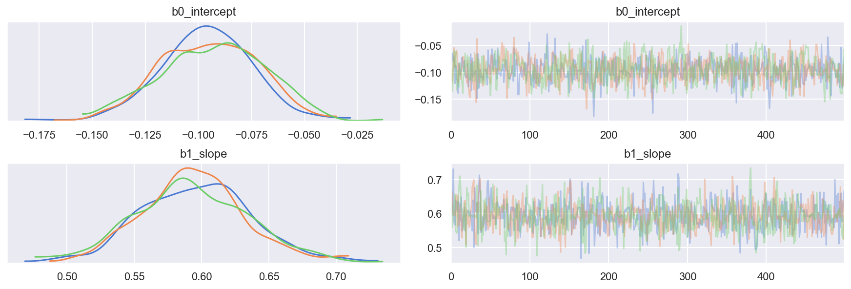
3.2.2 View Diagnostics
NOTE: We will illustrate the posterior OLS fit and compare to the datapoints in the final comparison plot
Traceplot
_ = az.plot_trace(trc_ols, combined=False, compact=False)
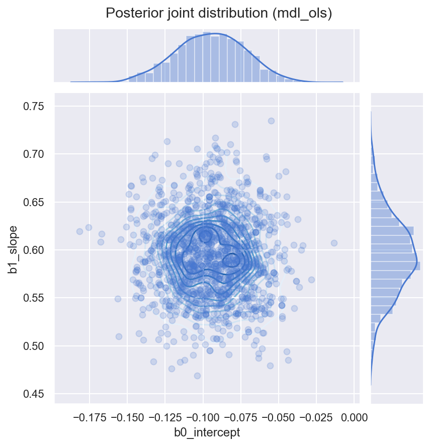
View posterior joint distribution (since the model has only 2 parameters, we can easily view this as a 2D joint distribution)
df_trc_ols = pm.trace_to_dataframe(trc_ols)
gd = sns.jointplot(x='b0_intercept', y='b1_slope', data=df_trc_ols, height=6,
                   marginal_kws={'kde':True, 'kde_kws':{'cut':1}},
                   joint_kws={'alpha':0.2})
gd.plot_joint(sns.kdeplot, zorder=0, cmap="Blues", n_levels=12)
_ = gd.fig.suptitle('Posterior joint distribution (mdl_ols)', y=1.02)
4. Simple Linear Model with Robust Student-T Likelihood
I’ve added this brief section in order to directly compare the Student-T based method exampled in Thomas Wiecki’s notebook in the PyMC3 documentation
Instead of using a Normal distribution for the likelihood, we use a Student-T which has fatter tails. In theory this allows outliers to have a smaller influence in the likelihood estimation. This method does not produce inlier / outlier flags (it marginalizes over such a classification) but it’s simpler and faster to run than the Signal Vs Noise model below, so a comparison seems worthwhile.
4.1 Specify Model
In this modification, the single likelihood is more robust to outliers:
ˆy∼StudentT(βT→xi,σi,ν)
where:
- β = {1,βj∈Xj} <— linear coefs in
Xj, in this case
1 + x - σ = noise term <— in this case we set this to an unpooled σi: the measured error
sigma_yfor each datapoint - ν = degrees of freedom <— allowing a pdf with fat tails and thus less influence from outlier datapoints
with pm.Model() as mdl_studentt:

    # define weakly informative Normal priors to give Ridge regression
    b0 = pm.Normal('b0_intercept', mu=0, sd=10)
    b1 = pm.Normal('b1_slope', mu=0, sd=10)

    # define linear model
    y_est = b0 + b1 * dfhoggs['x']

    # define prior for StudentT degrees of freedom
    # InverseGamma has nice properties:
    # it's continuous and has support x ∈ (0, inf)
    nu = pm.InverseGamma('nu', alpha=1, beta=1)

    # define Student T likelihood
    likelihood = pm.StudentT('likelihood', mu=y_est,
                             sigma=dfhoggs['sigma_y'], nu=nu,
                             observed=dfhoggs['y'])

pm.model_to_graphviz(mdl_studentt)

4.2 Fit Model
4.2.1 Sample Posterior
with mdl_studentt:
    trc_studentt = pm.sample(tune=5000, draws=500, chains=3, cores=3,
                    init='advi+adapt_diag', n_init=50000, progressbar=True)
Auto-assigning NUTS sampler...
Initializing NUTS using advi+adapt_diag...
Average Loss = 19.398:  31%|███▏      | 15631/50000 [00:11<00:24, 1417.33it/s]
Convergence achieved at 15700
Interrupted at 15,699 [31%]: Average Loss = 28.621
Multiprocess sampling (3 chains in 3 jobs)
NUTS: [nu, b1_slope, b0_intercept]
Sampling 3 chains: 100%|██████████| 16500/16500 [00:18<00:00, 905.18draws/s]
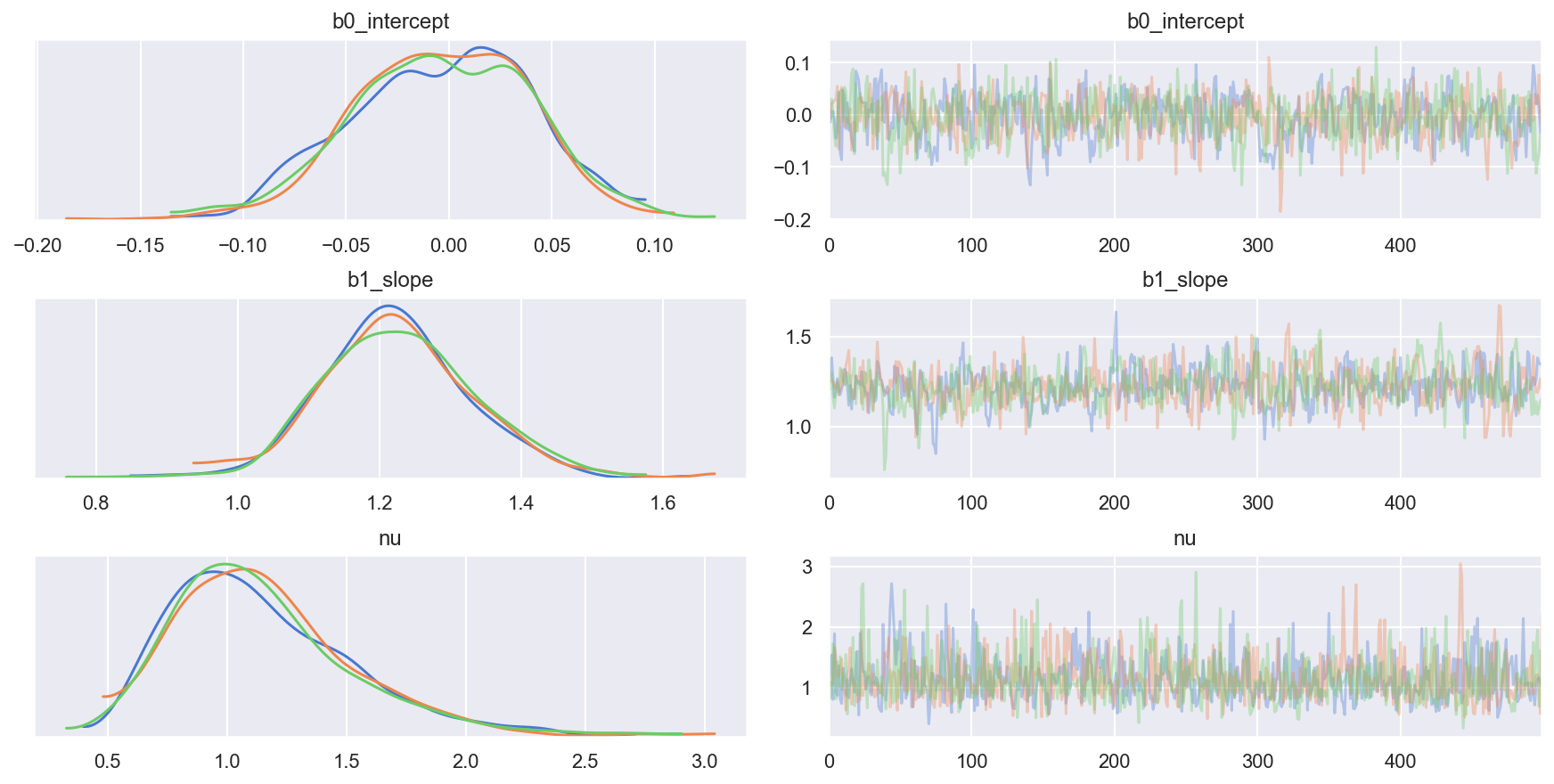
4.2.2 View Diagnostics
NOTE: We will illustrate this StudentT fit and compare to the datapoints in the final comparison plot
Traceplot
_ = az.plot_trace(trc_studentt, combined=False, compact=False)
4.2.3 View the shift in posterior joint distributions from OLS to StudentT
fts = ['b0_intercept', 'b1_slope']
df_trc = pd.concat((df_trc_ols[fts], df_trc_studentt[fts]), sort=False)
df_trc['model'] =  pd.Categorical(
                        np.repeat(['ols', 'studentt'], len(df_trc_ols)),
                        categories=['hogg_inlier', 'studentt', 'ols'],
                        ordered=True)

gd = sns.JointGrid(x='b0_intercept', y='b1_slope', data=df_trc, height=8)
_ = gd.fig.suptitle(('Posterior joint distributions' +
            '\n(showing general movement from OLS to StudentT)'), y=1.05)

_, x_bin_edges = np.histogram(df_trc['b0_intercept'], 60)
_, y_bin_edges = np.histogram(df_trc['b1_slope'], 60)

for idx, grp in df_trc.groupby('model'):
    _ = sns.scatterplot(grp['b0_intercept'], grp['b1_slope'],
                        ax=gd.ax_joint, alpha=0.2, label=idx)
    _ = sns.kdeplot(grp['b0_intercept'], grp['b1_slope'],
                        ax=gd.ax_joint, zorder=2, n_levels=7)
    _ = sns.distplot(grp['b0_intercept'], ax=gd.ax_marg_x, kde_kws={'cut':1},
                         bins=x_bin_edges, axlabel=False)
    _ = sns.distplot(grp['b1_slope'], ax=gd.ax_marg_y, kde_kws={'cut':1},
                         bins=y_bin_edges, vertical=True, axlabel=False)
_ = gd.ax_joint.legend()
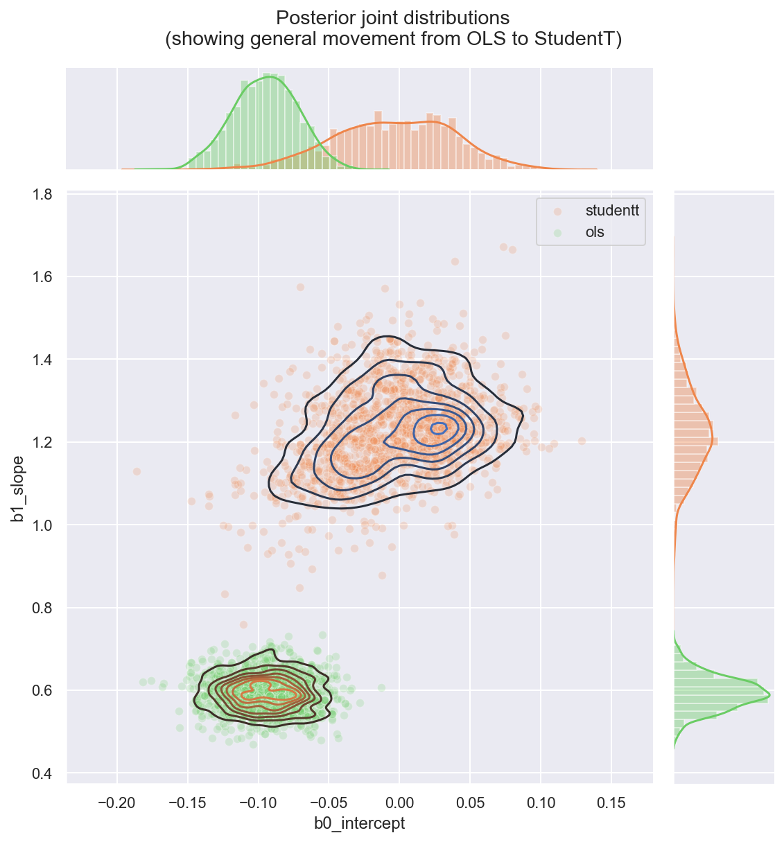
Observe:
- Both parameters
b0_interceptandb1_slopeappear to have greater variance than in the OLS regression - This is due to ν appearing to converge to a value
nu ~ 1, indicating that a fat-tailed likelihood has a better fit than a thin-tailed one - The parameter
b0_intercepthas moved much closer to 0, which is interesting: if the theoretical relationshipy ~ f(x)has no offset, then for this mean-centered dataset, the intercept should indeed be 0: it might easily be getting pushed off-course by outliers in the OLS model. - The parameter
b1_slopehas accordingly become greater: perhaps moving closer to the theoretical functionf(x)
5. Linear Model with Custom Likelihood to Distinguish Outliers: Hogg Method
Please read the paper (Hogg 2010) and Jake Vanderplas' code for more complete information about the modelling technique.
As noted above, the general idea is to create a ‘mixture’ model whereby datapoints can be described by either:
- the proposed (linear) model (thus a datapoint is an inlier), or
- a second model, which for convenience we also propose to be linear, but allow it to have a different mean and variance (thus a datapoint is an outlier)
5.1 Specify Model
The likelihood is evaluated over a mixture of two likelihoods, one for ‘inliers’, one for ‘outliers’. A Bernouilli distribution is used to randomly assign datapoints in N to either the inlier or outlier groups, and we sample the model as usual to infer robust model parameters and inlier / outlier flags:
logL=i=N∑ilog[(1−Bi)√2πσ2inexp(−(xi−μin)22σ2in)]+i=N∑ilog[Bi√2π(σ2in+σ2out)exp(−(xi−μout)22(σ2in+σ2out))]
where:
- Bi is Bernoulli-distibuted Bi∈{0(inlier),1(outlier)}
- μin=βT→xi as before for inliers, where β = {1,βj∈Xj} <— linear coefs in
Xj, in this case
1 + x - σin = noise term <— in this case we set this to an unpooled σi: the measured error
sigma_yfor each datapoint - μout <— is a random pooled variable for outliers
- σout = additional noise term <— is a random unpooled variable for outliers
with pm.Model() as mdl_hogg:

    # get into the practice of stating input data as Theano shared vars
    tsv_x = pm.Data('tsv_x', dfhoggs['x'])                                        # (n, )
    tsv_y = pm.Data('tsv_y', dfhoggs['y'])                                        # (n, )
    tsv_sigma_y = pm.Data('tsv_sigma_y', dfhoggs['sigma_y'])                      # (n, )

    # weakly informative Normal priors (L2 ridge reg) for inliers
    b0 = pm.Normal('b0_intercept', mu=0, sigma=10, testval=pm.floatX(0.1))
    b1 = pm.Normal('b1_slope', mu=0, sigma=10, testval=pm.floatX(1.))

    # linear model for mean for inliers
    y_est_in = b0 + b1 * tsv_x                                                    # (n, )

    # proposed mean for all outliers
    y_est_out = pm.Normal('y_est_out', mu=0, sigma=10, testval=pm.floatX(1.))     # (1, )

    # weakly informative prior for additional variance for outliers
    sigma_y_out = pm.HalfNormal('sigma_y_out', sigma=1, testval=pm.floatX(1.))    # (1, )

    # create in/outlier distributions to get a logp evaluated on the observed y
    # this is not strictly a pymc3 likelihood, but behaves like one when we
    # evaluate it within a Potential (which is minimised)
    inlier_logp = pm.Normal.dist(mu=y_est_in,
                                 sigma=tsv_sigma_y).logp(tsv_y)

    outlier_logp = pm.Normal.dist(mu=y_est_out,
                                  sigma=tsv_sigma_y + sigma_y_out).logp(tsv_y)

    # Bernoulli in/outlier classification constrained to [0, .5] for symmetry
    frac_outliers = pm.Uniform('frac_outliers', lower=0.0, upper=.5)
    is_outlier = pm.Bernoulli('is_outlier', p=frac_outliers,
                      shape=tsv_x.eval().shape[0],
                      testval=(np.random.rand(tsv_x.eval().shape[0]) < 0.4) * 1)  # (n, )

    # non-sampled Potential evaluates the Normal.dist.logp's
    potential = pm.Potential('obs', ((1-is_outlier) * inlier_logp).sum() +
                             (is_outlier * outlier_logp).sum())
5.2 Fit Model
5.2.1 Sample Posterior
Note that pm.sample conveniently and automatically creates the compound sampling process to:
- sample a Bernoulli variable (the class
is_outlier) using a discrete sampler - sample the continuous variables using a continous sampler
Further note:
- This also means we can’t initialise using ADVI, so will init using
jitter+adapt_diag - In order to pass
kwargsto a particular stepper, wrap them in a dict addressed to the lowercased name of the stepper e.g.nuts={'target_accept': 0.85} - This caught me out during development, because this commit (created in 2018 in response to this issue) removed the docstring for
step_kwargs, and that used to explain that kwargs should be addressed to the stepper
with mdl_hogg:
    trc_hogg = pm.sample(tune=6000, draws=500, chains=3, cores=3,
                         init='jitter+adapt_diag', nuts={'target_accept':0.9})
Multiprocess sampling (3 chains in 3 jobs)
CompoundStep
>NUTS: [frac_outliers, sigma_y_out, y_est_out, b1_slope, b0_intercept]
>BinaryGibbsMetropolis: [is_outlier]
Sampling 3 chains: 100%|██████████| 19500/19500 [00:43<00:00, 449.14draws/s]
5.2.2 View Diagnostics
NOTE: We will illustrate this model fit and compare to the datapoints in the final comparison plot
Traceplot
rvs = ['b0_intercept', 'b1_slope', 'y_est_out', 'sigma_y_out', 'frac_outliers']
_ = az.plot_trace(trc_hogg, var_names=rvs, combined=False)
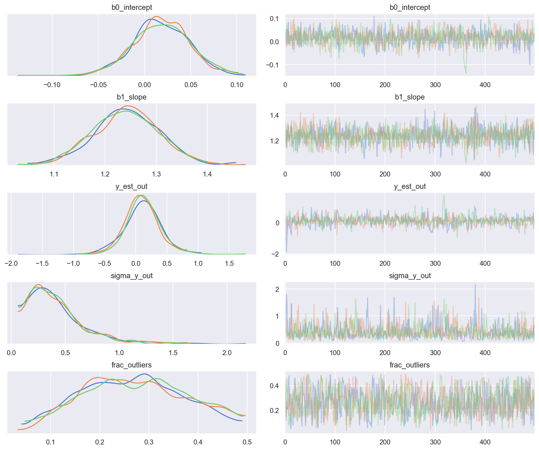
Observe:
- At the default
target_accept = 0.8there are lots of divergences, indicating this is not a particularly stable model - However, at
target_accept = 0.9(and increasingtunefrom 5000 to 6000), the traces exhibit fewer divergences and appear slightly better behaved. - The traces for the inlier model parameters
b0_interceptandb1_slope, and for outlier model parametery_est_out(the mean) look reasonably converged - The traces for outlier model param
y_sigma_out(the additional pooled variance) occasionally go a bit wild - I’m slightly peturbed that
frac_outliersis so dispersed: that’s quite a flat distribution: suggests that there are a few datapoints where their inliner/outlier status is subjective - Indeed as Thomas noted in his v2.0 Notebook, because we’re explicitly modeling the latent label (inlier/outliner) as binary choice the sampler could have a problem - rewriting this model into a marginal mixture model would be better.
Simple trace summary inc rhat
pm.summary(trc_hogg, var_names=rvs)
| mean | sd | mc_error | hpd_2.5 | hpd_97.5 | n_eff | Rhat | |
|---|---|---|---|---|---|---|---|
| b0_intercept | 0.017191 | 0.031101 | 0.001042 | -0.047390 | 0.074615 | 793.464520 | 0.999149 |
| b1_slope | 1.240391 | 0.064382 | 0.001987 | 1.110171 | 1.360046 | 1147.170130 | 1.000458 |
| y_est_out | 0.104516 | 0.291202 | 0.010213 | -0.498045 | 0.670796 | 760.256224 | 1.005919 |
| sigma_y_out | 0.423364 | 0.273111 | 0.008358 | 0.063661 | 0.929918 | 855.002935 | 0.999450 |
| frac_outliers | 0.270572 | 0.104870 | 0.003415 | 0.080593 | 0.465110 | 830.279459 | 1.000730 |
5.2.3 View the shift in posterior joint distributions from OLS to StudentT to Hogg
fts = ['b0_intercept', 'b1_slope']
df_trc = pd.concat((df_trc_ols[fts], df_trc_studentt[fts], df_trc_hogg), sort=False)
df_trc['model'] = pd.Categorical(
                    np.repeat(['ols', 'studentt', 'hogg_inlier'], len(df_trc_ols)),
                    categories=['hogg_inlier', 'studentt', 'ols'], ordered=True)

gd = sns.JointGrid(x='b0_intercept', y='b1_slope', data=df_trc, height=8)
_ = gd.fig.suptitle(('Posterior joint distributions' +
            '\nOLS, StudentT, and Hogg (inliers)'), y=1.05)

_, x_bin_edges = np.histogram(df_trc['b0_intercept'], 60)
_, y_bin_edges = np.histogram(df_trc['b1_slope'], 60)

for idx, grp in df_trc.groupby('model'):
    _ = sns.scatterplot(grp['b0_intercept'], grp['b1_slope'],
                        ax=gd.ax_joint, alpha=0.2, label=idx)
    _ = sns.kdeplot(grp['b0_intercept'], grp['b1_slope'],
                        ax=gd.ax_joint, zorder=2, n_levels=7)
    _ = sns.distplot(grp['b0_intercept'], ax=gd.ax_marg_x, kde_kws={'cut':1},
                         bins=x_bin_edges, axlabel=False)
    _ = sns.distplot(grp['b1_slope'], ax=gd.ax_marg_y, kde_kws={'cut':1},
                         bins=y_bin_edges, vertical=True, axlabel=False)
_ = gd.ax_joint.legend()
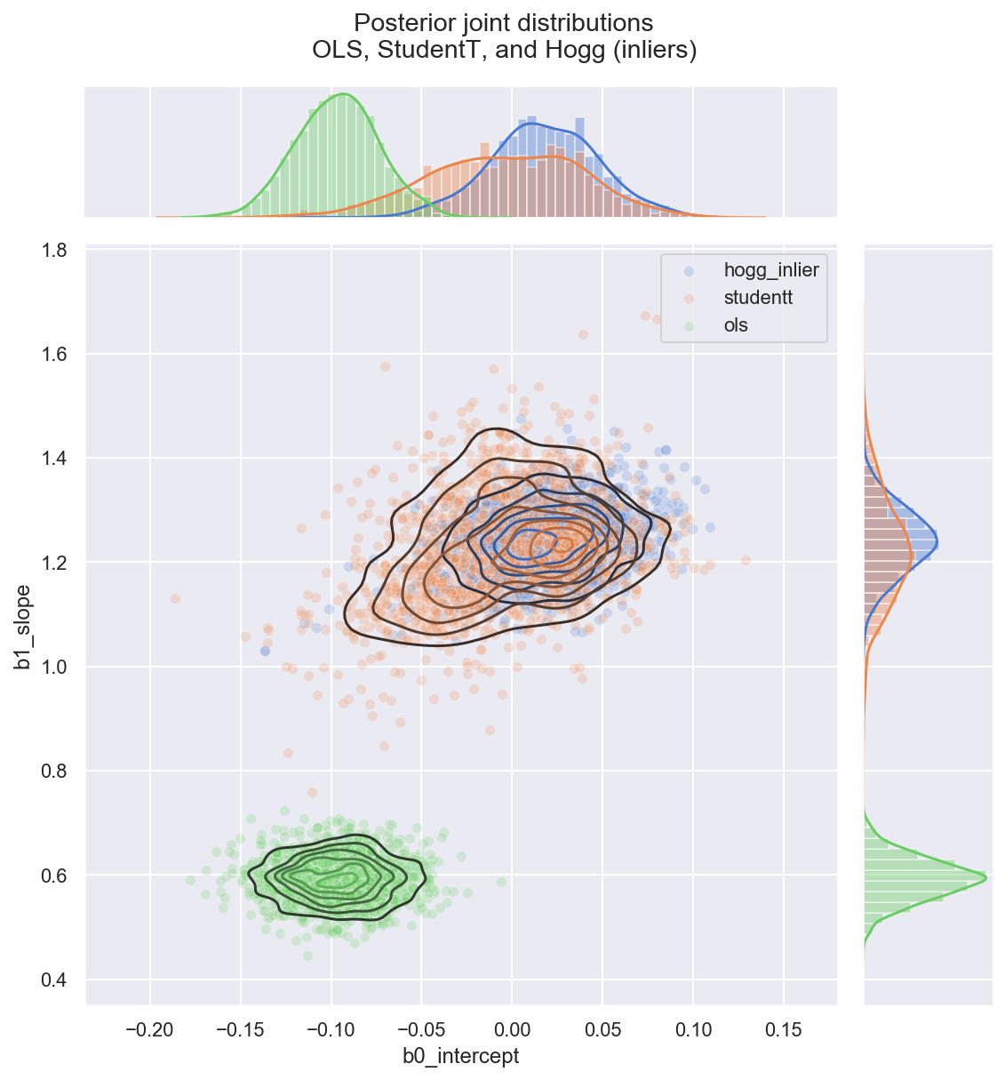
Observe:
- The
hogg_inlierandstudenttmodels converge to similar ranges forb0_interceptandb1_slope, indicating that the (unshown)hogg_outliermodel might perform a similar job to the fat tails of thestudenttmodel: allowing greater log probability in awway from the main linear distribution in the datapoints - As expected, (since it’s a Normal) the
hogg_inlierposterior has thinner tails and more probability mass concentrated about the central values - The
hogg_inliermodel also appears to have moved farther away from both theolsandstudenttmodels on theb0_intercept, suggesting that the outliers really distoring that particular dimension
5.3 Declare Outliers
5.3.1 View ranges for inliers / outlier predictions
At each step of the traces, each datapoint may be either an inlier or outlier. We hope that the datapoints spend an unequal time being one state or the other, so let’s take a look at the simple count of states for each of the 20 datapoints.
df_outlier_results = pd.DataFrame.from_records(trc_hogg['is_outlier'],
                                               columns=dfhoggs.index)
dfm_outlier_results = pd.melt(df_outlier_results,
                              var_name='datapoint_id', value_name='is_outlier')

gd = sns.catplot(y='datapoint_id', x='is_outlier', data=dfm_outlier_results,
                 kind='point', join=False, height=6, aspect=2)
_ = gd.fig.axes[0].set(xlim=(-0.05,1.05), xticks=np.arange(0, 1.1, 0.1))
_ = gd.fig.axes[0].axvline(x=0, color='b', linestyle=':')
_ = gd.fig.axes[0].axvline(x=1, color='r', linestyle=':')
_ = gd.fig.axes[0].yaxis.grid(True, linestyle='-', which='major',
                              color='w', alpha=0.4)
_ = gd.fig.suptitle(('For each datapoint, distribution of outlier classification '+
                    'over the trace'), y=1.04, fontsize=16)
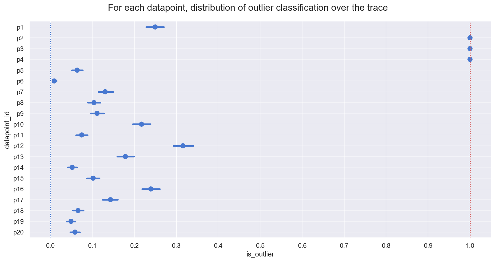
Observe:
- The plot above shows the proportion of samples in the traces in which each datapoint is marked as an outlier, expressed as a percentage.
- 3 points [p2, p3, p4] spend >=95% of their time as outliers
- Note the mean posterior value of
frac_outliers ~ 0.27, corresponding to approx 5 or 6 of the 20 datapoints: we might investigate datapoints[p1, p10, p12, p16]to see if they lean towards being outliers
The 95% cutoff we choose is subjective and arbitrary, but I prefer it for now, so let’s declare these 3 to be outliers and see how it looks compared to Jake Vanderplas' outliers, which were declared in a slightly different way as points with means above 0.68.
5.3.2 Declare outliers
Note:
- I will declare outliers to be datapoints that have value == 1 at the 5-percentile cutoff, i.e. in the percentiles from 5 up to 100, their values are 1.
- Try for yourself altering cutoff to larger values, which leads to an objective ranking of outlier-hood.
cutoff = .05
dfhoggs['classed_as_outlier'] = np.quantile(trc_hogg['is_outlier'], cutoff, axis=0) == 1
dfhoggs['classed_as_outlier'].value_counts()
False    17
True      3
Name: classed_as_outlier, dtype: int64
Also add flag for points to be investigated. Will use this to annotate final plot
dfhoggs['annotate_for_investigation'] = np.quantile(trc_hogg['is_outlier'],
                                                    0.75, axis=0) == 1
dfhoggs['annotate_for_investigation'].value_counts()
False    16
True      4
Name: annotate_for_investigation, dtype: int64
5.4 Posterior Prediction Plots for OLS vs StudentT vs Hogg “Signal vs Noise”
gd = sns.FacetGrid(dfhoggs, height=10, hue='classed_as_outlier',
                   hue_order=[True, False], palette='Set1', legend_out=False)

# plot hogg outlier posterior distribution
outlier_mean = lambda x, s: s['y_est_out'] * x ** 0
pm.plot_posterior_predictive_glm(trc_hogg, lm=outlier_mean,
            eval=np.linspace(-3, 3, 10), samples=400,
            color='#CC4444', alpha=.2, zorder=1)

# plot the 3 model (inlier) posterior distributions
lm = lambda x,s: s['b0_intercept'] + s['b1_slope'] * x

pm.plot_posterior_predictive_glm(trc_ols, lm=lm,
            eval=np.linspace(-3, 3, 10), samples=200,
            color='#22CC00', alpha=.3, zorder=2)

pm.plot_posterior_predictive_glm(trc_studentt, lm=lm,
            eval=np.linspace(-3, 3, 10), samples=200,
            color='#FFA500', alpha=.5, zorder=3)

pm.plot_posterior_predictive_glm(trc_hogg, lm=lm,
            eval=np.linspace(-3, 3, 10), samples=200,
            color='#357EC7', alpha=.5, zorder=4.)
_ = plt.title(None)

line_legend = plt.legend(
    [Line2D([0], [0], color='#357EC7'), Line2D([0], [0], color='#CC4444'),
    Line2D([0], [0], color='#FFA500'), Line2D([0], [0], color='#22CC00')],
    ['Hogg Inlier', 'Hogg Outlier', 'Student-T', 'OLS'], loc='lower right',
    title='Posterior Predictive')
_ = gd.fig.get_axes()[0].add_artist(line_legend)

# plot points
_ = gd.map(plt.errorbar, 'x', 'y', 'sigma_y', 'sigma_x', marker="o",
          ls='', markeredgecolor='w', markersize=10, zorder=5).add_legend()
_ = gd.ax.legend(loc='upper left', title='Outlier Classification')

# annotate the potential outliers
for idx, r in dfhoggs.loc[dfhoggs['annotate_for_investigation']].iterrows():
    _ = gd.axes.ravel()[0].annotate(s=idx, xy=(r['x'], r['y']), xycoords='data',
            xytext=(7, 7), textcoords='offset points', color='#999999', zorder=4)

## create xlims ylims for plotting
x_ptp = np.ptp(dfhoggs['x'].values) / 3.3
y_ptp = np.ptp(dfhoggs['y'].values) / 3.3
xlims = (dfhoggs['x'].min()-x_ptp, dfhoggs['x'].max()+x_ptp)
ylims = (dfhoggs['y'].min()-y_ptp, dfhoggs['y'].max()+y_ptp)
_ = gd.axes.ravel()[0].set(ylim=ylims, xlim=xlims)
_ = gd.fig.suptitle(('Standardized datapoints in Hogg 2010 dataset, showing ' +
        'posterior predictive fit for 3 models:\nOLS, StudentT and Hogg ' +
        '"Signal vs Noise" (inlier vs outlier, custom likelihood)'),
                    y=1.04, fontsize=16)
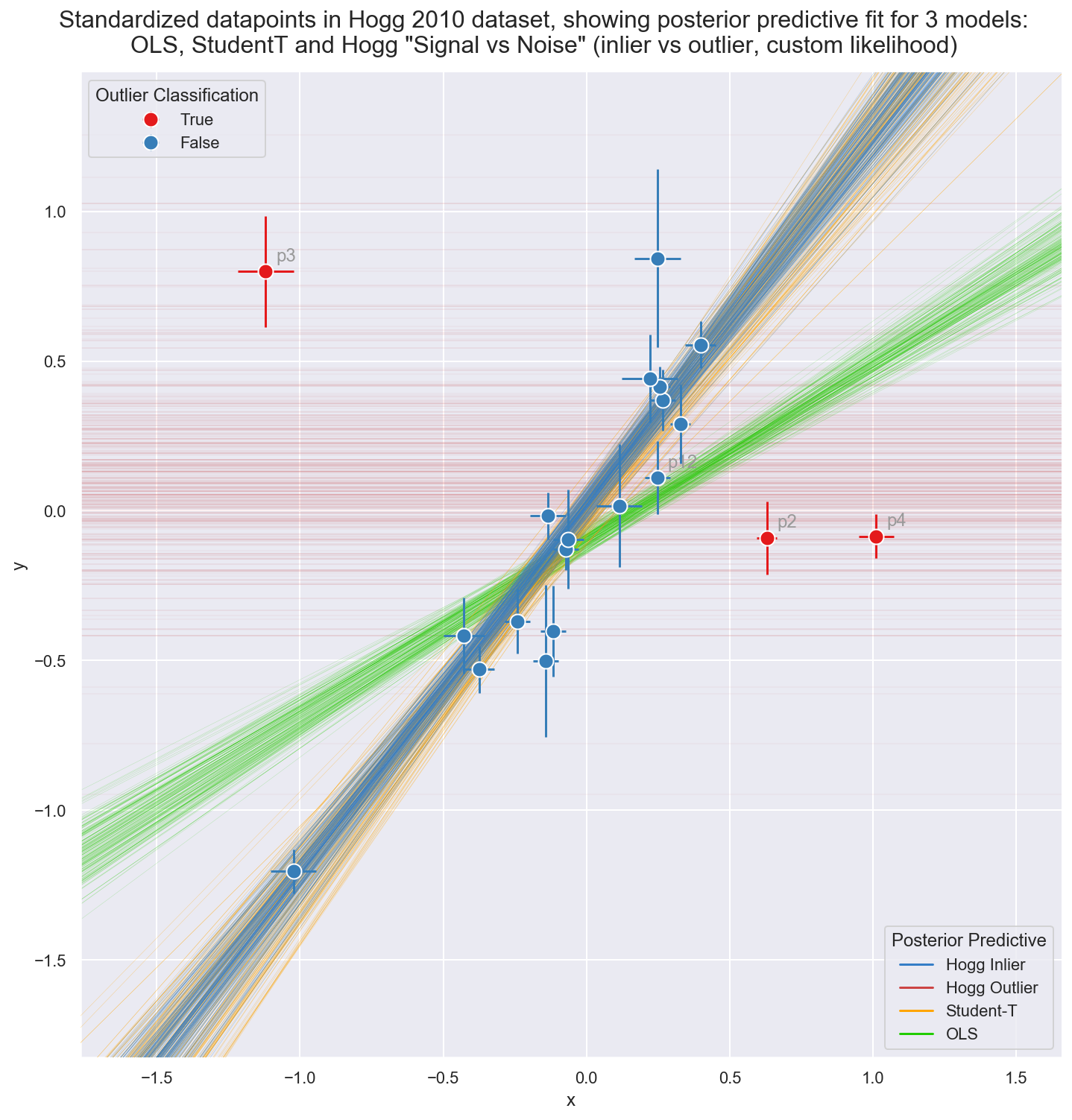
Observe:
The posterior preditive fit for:
- the OLS model is shown in Green and (as expected) it doesn’t appear to fit the majority of our datapoints very well: skewed by outliers
- the Student-T model is shown in Orange and does appear to fit the ‘main axis’ of datapoints quite well, ignoring outliers
- the Hogg Signal vs Noise model is shown in two parts:
- Blue for inliers fits the ‘main axis’ of datapoints well, ignoring outliers
- Red for outliers has a very large variance and has assigned ‘outlier’ points with more log likelihood than the Blue inlier model
We see that the Hogg Signal vs Noise model also yields specific estimates of which datapoints are outliers:
- 17 ‘inlier’ datapoints, in Blue and
- 3 ‘outlier’ datapoints shown in Red.
- From a simple visual inspection, the classification seems fair, and agrees with Jake Vanderplas' findings.
- I’ve annotated these Red outliers and the most outlying inliers
[p1, p12, p16]to aid visual investigation
Overall:
- the Hogg Signal vs Noise model behaves as promised, yielding a robust regression estimate and explicit labelling of inliers / outliers, but
- the Hogg Signal vs Noise model is quite complex, and whilst the regression seems robust, the traceplot shoes many divergences, and the model is potentially unstable
- if you simply want a robust regression without inlier / outlier labelling, the Student-T model may be a good compromise, offering a simple model, quick sampling, and a very similar estimate.
Postscript
If you made it this far, great! This is an attempt to mix a blogpost with a technical notebook in the style of a mini case study. The code is valid and extracted verbatim from the full Notebook, but these are excerpts, and to fully reproduce you should use the Notebook.
There’s a back catalogue of this material that I plan to overhaul and release
over coming weeks, some to the pymc3_examples repo, some to project-specific
repos, and contributing to the PyMC3 project docs where possible.
Further Note
Very nice to see Dan Foreman-Mackey
chime in via Twitter to note his
alternative marginalised likelihood in pymc3
using the same setup and dataset! I plan to do a followup Notebook using an
explicit GMM class via pm.Mixture and pm.NormalMixture, so will compare
there too. I also appreciate
the link to Dan’s earlier implementation
of this Hogg model using his emcee
package which is one of the first MCMC packages I worked with on a client
project way back in 2014. Nice one Dan
(and thanks Thomas for the initial tweet).
The power of the internet, eh?