Editor’s note: this post is from The Sampler archives in 2015. During the last 4 years a lot has changed, not least that now most companies in most sectors have contracted / employed data scientists, and built / bought / run systems and projects. Most professionals will at least have an opinion now on data science, occasionally earned.

Let’s see how well this post has aged - feel free to comment below - and I might write a followup at some point.

In this series of blogposts we’ll explain tools & techniques of dealing with time-to-event data, and demonstrate how survival analysis is integral to many business processes.

Survival analysis is long established within actuarial science and medical research but seems infrequently used in general data science projects. In this series of blogposts we will:

• introduce survival analysis as a vital technique in any statisticians toolkit
• demonstrate a general approach to undertaking a data science project: accessing, cleaning and storing data, and using a range of open-source analytical tools that enable rapid iteration, data exploration, modelling and visualisation
• use a real-world dataset and seek to both match and improve upon some existing analysis already undertaken and released by a third-party.

By the end you should have a better understanding of the theory, some tools and techniques, and hopefully gain some ideas about how survival analysis can be applied to all manner of event-based processes that are often crucial to business operations.

A Quick Definition and Some Examples

Wikipedia defines survival analysis as:

a branch of statistics that deals with analysis of time duration until one or more events happen, such as death in biological organisms and failure in mechanical systems.

We might for example, expect a life actuary to try to predict what proportion of the general population will survive past a certain age¹. She might furthermore want to know the ‘rate of change of survival’ (the hazard function), and the characteristics of individuals which most influence their survival.

More generally, we can use survival analysis to model the expected time-to-event for a wide variety of situations:

• User shopping behaviour <— e.g. the elapsed time between a user subscribing to an online shopping service and ordering their first product
• Crop yields and harvesting <— e.g. the duration between seeding a field and the majority of the crops being ready for harvest
• Radioactive halflife <— e.g. the time until half the atoms in a luminous blob² of tritium have decayed into hydrogen and helium-3
• Hardware failure rates <— e.g. the lifetime for a piece of machinery before component failure
• Customer subscription persistence <— e.g. the time for a customer to remain subscribed to a cellphone service before churning
• Claims settlement time <— e.g. the duration between an insurance claim being notified and fully paid closed (and also the shorter durations between stages within that business process)

A worked example: truck maintenance scheduling

Imagine we have a fleet of haulage trucks and we’re particularly interested in the elapsed time between purchase and first maintenance event (aka repairs aka servicing).

We could use this analysis to:

• Identify which manufacturers and models of trucks require the least repair and favour buying those again in future
• Identify contributing factors leading to trucks needing earlier repairs and try to mitigate issues
• Anticipate likely spikes of activity for fleet repair during the year and ensure funds are available in advance

The following sections refer to this example.

The Basics

Plot a survival curve

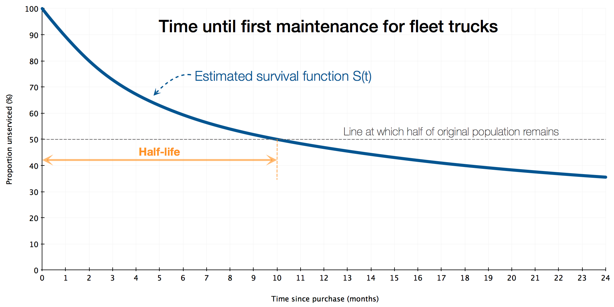
Observe:

• The relative duration of our study is measured from time of purchase until the end of the second year (24 months) - this is a relative time and will likely begin at a different real-time for each truck
• The survival function is a measure of how many trucks are serviced at each point in relative-time. It drops quickly and then flattens out; it crosses the 50% line at 10 months, meaning that by 10 months we can expect 50% of all the trucks in the fleet to have had their first service.
• About 36% of trucks remain unserviced at the end of the first 24 months; conversely, about 64% will have a service event during their first 24 months

The survival function $S(t)$

The survival function, $S(t)$, of an individual is the probability that they survive until at least time $t$.

$$ \begin{align} S(t) = P(T > t) \end{align} $$

…where $t$ is a time of interest and $T$ is the time of event.

The survival curve is non-increasing (the event may not reoccur for an individual) and is limited within the range $[0,1]$.

Note:

• that the event might not happen within our period of study and we call this right-censoring. This happens in the above example where for 36% of trucks, all we know is that their first service happens some time after 24 months
• we can’t state exactly which truck will experience the event, nor exactly when the event will occur, we only work with the aggregate values.

The half-life $t_{\frac{1}{2}}$

We saw the half-life of truck repair illustrated above (the orange arrows). Most people are familiar with measuring this:

1. select a group of individuals - our fleet of trucks - and measure how long it takes for the event of interest to occur
2. once the event of interest - the first service repair - occurs for half of the population, that period is aka the half-life

There’s nothing particularly special about the half-life, and we might be interested in the time taken for e.g. 25% of the trucks to come in for first service, or 75% or 90% etc.

The hazard function $\lambda(t)$

The hazard function (aka decay function) $\lambda(t)$ is related to the survival function, and tells us the probability that the event $T$ occurs in the next instant $t + \delta t$, given that the individual has reached timestep $t$:

$$ \begin{align} \lambda(t) = \lim_{\delta{t} \rightarrow 0} \frac{\Pr(t \leq T < t + \delta t \ | \ T > t)}{\delta{t}} \end{align} $$

With some maths³ one can work back to the survival function $S(t)$:

$$ \begin{align} S(t) = exp(- \int\limits_{0}^{t} \lambda(u)du) \end{align} $$

The hazard function $\lambda(t)$ is non-parametric, so we can fit a pattern of events that is not necessarily monotonic.

Other measurements and important considerations

The cumulative hazard function

An alternative representation of the time-to-event behaviour is the cumulative hazard function $\Lambda(t)$, which is essentially the summing of the hazard function over time, and is used by some models for its greater stability.

We can show:

$$ \begin{align} \Lambda(t) &= \int\limits_{0}^{t} \lambda(u)du \newline &= -\log S(t) \end{align} $$

… and the simple relation of $\Lambda(t)$ to the survival function $S(t)$ is a nice property, exploited in particular by the Cox Proportional Hazards and Aalen Additive models, which we’ll demonstrate later.

Stating it slightly differently, we can parametrically relate the attributes of the individuals to their survival curve:

$$ \begin{align} S(t) = -e^{\sum \Lambda_i(t)} \end{align} $$

This powerful approach is known as Survival Regression. In the trucks example, we might want to know the relative impact of engine size, hours of service, geographical regions driven etc upon the time from first purchase to first service.

Censoring and truncation

We’re measuring time-to-event in the real world and so there’s practical constraints on the period of study and how to treat individuals that fall outside that period. Censoring is when the event of interest (repair, first sale, etc) occurs outside the study period, and truncation is due to the study design.

The following discussion continues our hypothetical truck maintenance study:

• We imagine that our data source is a set of database extracts taken at the start of 2014 for a 3-year period from mid-2010 to mid-2013, and this is all of the data we could extract from the company database

• It may be that we have very little data about service-intervals longer than 24 months, so despite the study period covering 36 months, when we calculate survival curves we decide to only look at the first 24 months of a trucks life

• All trucks remain in daily operation through end-2014, none are sold or scrapped.

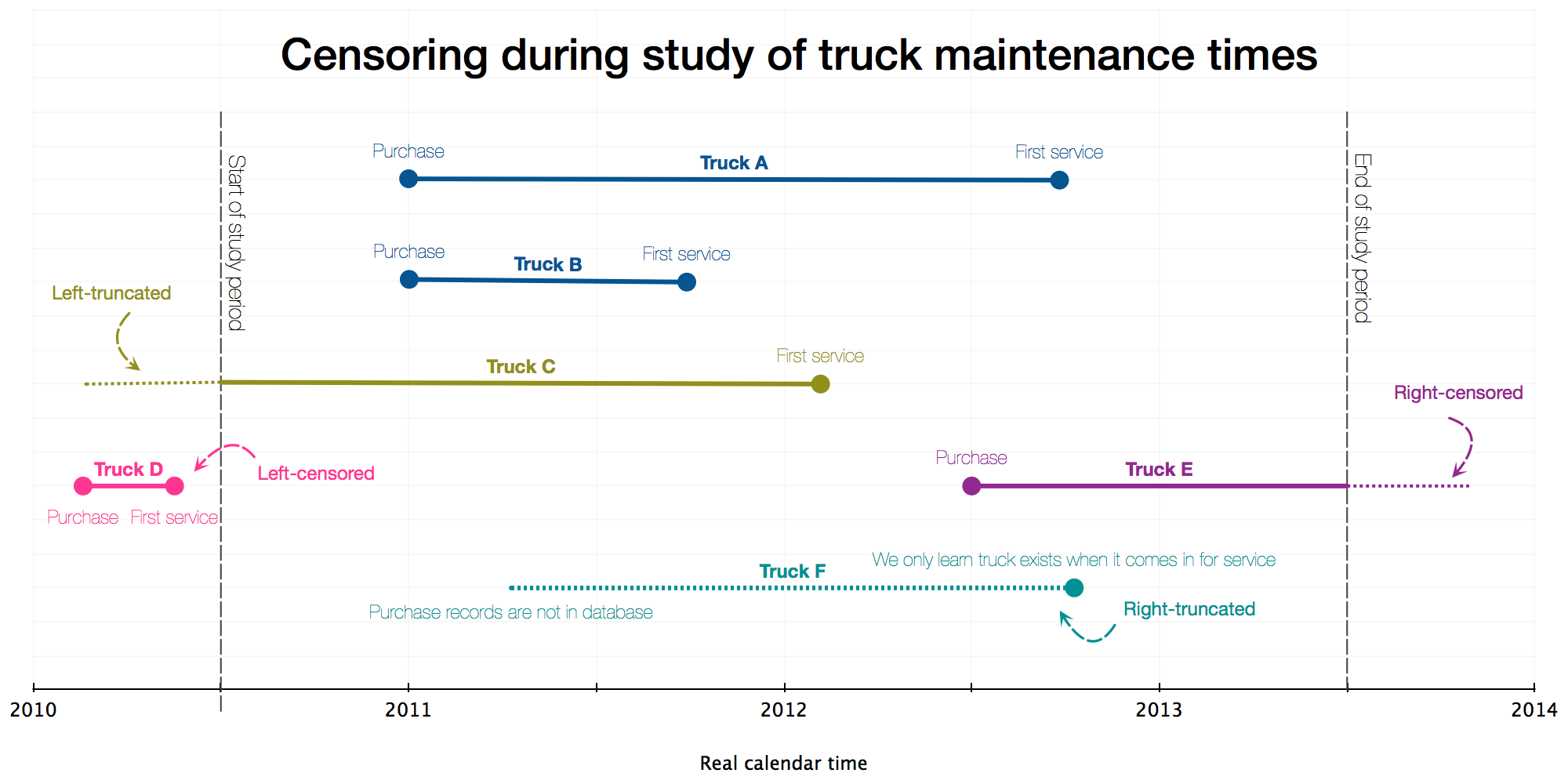
Observe:

• Truck A was purchased at start-2011 and first serviced 21 months later. It has a first-service-period or ‘survival’ of 21 months

• Truck B was also purchased at start-2011 but first serviced 9 months later. This 9-month survival is much shorter than for Truck A: perhaps it has a different manufacturer or was driven differently. The various survival models let us explore these factors in different ways

• Truck C was first serviced in Feb 2012, but purchased prior to the start of our study period. This left-truncation is a consequence of our decision to start the study period at mid-2010, and we may mitigate by adjusting the start of the study period or adjusting the lifetime value of the truck

• Truck D was purchased in Feb 2010 and serviced soon afterwards - both prior to the study period - so we did not observe the service event during the study. In fact, if we’re strict about our data sampling then we wouldn’t even know about this event from our database extract. The need to account for such left-censoring is rarely encountered in practice

• Truck E was purchased in Jun 2012 and by the end of the study in mid-2013 it had still not gone for first service. This right-censoring is very common in survival analysis

• Truck F does not appear at all in the purchases database and the first time we learn it exists is from the record of its first maintenance service during

2012. We are unlikely to encounter such right-truncation in practice, since we’re dealing with well-kept database records for purchases.

Censoring and truncation differ from one analysis to the next and it’s always vitally important to understand the limitations of the study and state the heuristics used. Generally, one can expect to deal often with right-censoring, occasionally with left-truncation, and very rarely with left-censoring or right-truncation.

What models can we use?

The very simplest survival models are really just tables of event counts: non-parametric, easily computed and a good place to begin modelling to check assumptions, data quality and end-user requirements etc.

Kaplan-Meier Model

This model gives us a maximum-likelihood estimate of the survival function $\hat S(t)$ like that shown in the first diagram above.

$$ \begin{align} \hat{S}(t) = \prod\limits_{t_{i} < t} \frac{n_i - d_i}{n_i} \end{align} $$

where:

• $d$ is the count of ‘death’ events
• $n$ is the count of individuals at risk at timestep $i$

The cumulative product gives us a non-increasing curve where we can read off, at any timestep during the study, the estimated probability of survival from the start to that timestep. We can also compute the estimated survival time or median survival time (half-life) as shown above.

Nelson-Aalen Model

A close alternative method is the Nelson-Aalen model, which estimates the cumulative hazard function $\Lambda(t) = -log S(t)$ and is more stable since it has a summation form:

$$ \begin{align} \hat \Lambda(t) = \sum\limits_{t_i\leq t} \frac{d_i}{n_i} \end{align} $$

where again:

• $d$ is the count of ‘death’ events
• $n$ is the count of individuals at risk at timestep $i$

This approach of estimating the hazard function is the basis for many more methods, including:

Cox Proportional Hazards Model

Having computed the survival function⁴ for a population, the logical next step is to understand the effects of different characteristics of the individuals. In our truck example above, we might want to know whether maintenance periods are affected more or less by mileage, or by types of roads driven, or the manufacturer, model or load-capacity of truck etc.

The Cox PH model is stated as an exponential decay model, yielding a semi-parametric method of estimating the hazard function at time $t$ given a baseline hazard that’s modified by a set of covariates:

$$ \begin{align} \lambda(t|X) &= \lambda_0(t) e^{\beta_1x_1 + \cdots + \beta_px_p} \newline &= \lambda_0(t) e^{\beta\vec{x}} \end{align} $$

where:

• $\lambda_0(t)$ is the non-parametric baseline hazard function
• $\beta\vec{x}$ is a linear parametric model using features of the individuals
• this ought to look familiar as an exponential decay of form: $N(t) = N_{0} e^{-\lambda t}$

We can now make comparative statements such as:

• “the hazard rate for trucks from manufacturer A is 2x greater than for manufacturer B”
• “trucks that drive 100 fewer km per week tend to have their first service up to 6 months later”
• etc etc

There’s many more models…

Survival analysis has been developed by many hands over many years and there’s an embarrassment of riches in the literature, including:

• Parametric / Accelerated Failure Time models, using various link functions including Exponential, Gompertz, Weibull, Log-logistic
• Aalen Additive models
• Bayesian inferential models

… but we’ll save the detail on those for specific examples in future posts in this series.

Final note

It takes a surprising amount of detail to explain the basics of survival analysis, so thank you for reading this far! As noted above, time-to-event analyses are very widely applicable to all sorts of real-world behaviours - not just studies of lifespan in actuarial or medical science.

In the rest of this series we’ll use a publicly available dataset to demonstrate implementing a survival model, interpreting the results, and we’ll try to learn something along the way.

---

1. Life insurance was amongst the first commercial endeavors of the modern era to use data analysis: with the first life tables compiled by the astronomer and physicist Edmond Halley in the 1690’s. Halley was involved in a surprising amount of analytical research, and as a contemporary of Flamsteed, Hooke, Wren and Newton he made a tremendous contribution to mathematics. This book is a good place to start. In the mid 1700’s mathematical tools were in place to allow Edward Rowe Mores to establish the world’s first mutual life insurer based on sound actuarial principles. ↩︎

2. If you have an old watch (pre-2000) with “T SWISS MADE T” somewhere on the dial, the T indicates that a luminous Tritium-containing compound is painted onto the hands and dial. You’ll probably also sadly notice that it’s completely failing to glow in the dark because the radioactive half-life of ~12.4 years means there’s very little Tritium left now. ↩︎

3. For a thorough but easily-digested derivation of survival and hazard functions, see the Wikipedia page. ↩︎

4. The survival, hazard and cumulative hazard functions are often mentioned seemingly-interchangeably in casual explanations of survival analysis, since usually if you have one function you can have the other(s). In our experience its best to present results to general audiences as a computed survival curve regardless of the model used. ↩︎